Lessons learnt from replaying ELB logs at scale

As part of our exercise of porting a Kotlin application to Go, we wanted to test the port by mirroring production traffic to it in lower environments. Our applications are hosted on AWS, and initially the platform team had considered VPC mirroring to accomplish this goal. However, the option turned out to be infeasible for reasons unbeknownst to me.

We resorted to replaying ELB log messages from one environment to another. This is a fairly common activity and we hoped to find a repository for the same on Github.

We came across the following Go projects for the purpose of playing ELB access logs.

• ONSdigital/aws-elb-replay
• AppsFlyer/elb-log-replay

The projects did not completely meet our requirements, but were a good starting point.

The first solution accepts log files from the previous day (the time frame can be configured), loops over the log messages creating a goroutine for each log entry. The goroutines sleep until it is time to send the request. So for example, at 1300 hrs if I process a log file containing a message from 1700 hrs yesterday it will create a goroutine that sleeps for 4 hours before sending the request. This technique works if you have a small number of requests. When we tried running the application with a few thousand log messages, it froze. And that was it. The solution did not seem scalable so we decided to explore the second option.

The latter is eleganlty designed. I urge you check the readme file in the repository. The authors have done a great job of documenting the architecture.

The following quote from the read me summarises how the player has been implemented.

To make this possible we chose a design pattern called pipelines also described here https://blog.golang.org/pipelines

• A single routine reads the log files and sends them one by one to a channel.
• On the other side of this channel there are num-senders routines that consume from that channel and for each log line they: parse the log line and synchronously send the request and wait for the response.

Eventually we collect the stats (actual rate and latency) and output them for monitoring puprposes. (sic)

The project provided us a robust foundation to build on. In this post I document five takeaways from working on enhancing AppsFlyer/elb-log-replay (hereafter referred to as the base project).

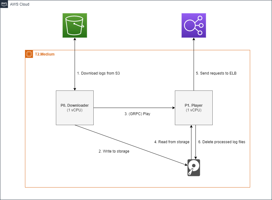
The downloader

The base project has been developed as a command line application. It accepts the path to a local directory and then sends each file present in the directory through the pipeline described above.

We needed to design a job that would fetch the log files from Amazon S3, process them (described in the next section), and then pass the list of files to the player.

We decided to strip away the command line interface of the base project and replace it with a shiny new GRPC server. At this point I’m sure I’ve managed to raise a few eyebrows by bringing GRPC into the design. We wanted to ensure that the downloader and the log player do not get into contention for CPU time. A simple solution was to separate the two into independent processes and specify their CPU allocation with GOMAXPROCS.

The approach allowed us to download log files and process them periodically while maintaining the desired throughput of the log player.

Traffic shaping

Before we could send the log files for replaying we had to weed out access logs of routes that we did not intend to replay. This took away any processing task that might have been needed by the base project.

Our Elastic Load Balancer instances are configured to generate log files at an interval of 5 minutes. As a first step we calculated the throughput using the following formula.

throughput = no_of_lines / ( 5 * 60 )

The filtered logs and the desired throughput were saved as two independent files and the parent directory was sent to the base project for replaying by the downloader every five minutes via GRPC.

A major limitation of this implementation was that we were not able to reproduce the traffic spikes we were seeing in production. Taking an average of five minutes was smoothing out momentary surges. We decided to split a five minute window into twenty quartiles, that helped us paint a picture closer to reality.

Scaling out

Having one compute instance simulate the traffic generated by tens or even hundreds of thousands of users is unrealistic. The system was designed keeping this in mind.

In fact, AWS’s way of saving a log file per ELB instance meant that all we had to do was to have one compute instance for each ELB instance.

This setup helped us easily achieve throughputs north of 700k requests per minute, with enough cpu and networking resources to spare.

Tuning the system for throughput

Getting the math right on calculating how much load a compute instance was able to generate was important. For example, if the response time of a request is about 20ms, we can have a throughput of only 50 requests per second per connection. If we have a connection pool of 5, we increase the throughput five-fold to 250 requests per second.

While configuring the pool size we encountered two gotchas.

• Each connection in the pool is represented by a file descriptor. While creating a pool of connections you are limited by the number of open file descriptors you are allowed to have. You can use uname -n to check and also set the limit.

• This gotcha is specific to Go. Even though you can set the connection pool size using the MaxIdleConns property, you will be limited to having only 2 connections per host unless you override the default value by setting MaxIdleConnsPerHost.

A big shout out to tleyden.github.io for documenting their findings in the blog post.

Deployment

Given that this tool would be seldom used, and possibly shelved once our transition from Kotlin to Go is complete meant we needed something simpler than having someone from the platform team configure a brand new pipeline for it.

For the first few runs we used the AWS CLI to provision resources, and then scp-ed the binaries and SSH-ed into the compute instances to start the applications. It was an onerous task.

Our first attempt at automating this was to write an elaborate bash script which soon turned ugly. Terraform provided a great way of provisioning and draining infrastructure resources, as well as deploying and executing our binaries.